.::howieko::.
Stuff that I'm learning
In this post, I’ll walk through building a deep learning neural network using PyTorch to identify 102 different species of flowers. This was the final project of the Udacity AI Programming with Python nanodegree.
The dataset was provided by Udacity, and I did all my model training using Jupyter Notebooks hosted on Paperspace.
Deep learning is new to me, and my learning approach has been to get exposed to as many resources as possible. So I’ll also be doing the same project, but using the Fastai library instead. I’ll post that when available.
For now, let’s go through the project using Pytorch. The text/content provided by Udacity are italicized. I’ve kept them in here for reference purposes.
Developing an AI application
Going forward, AI algorithms will be incorporated into more and more everyday applications. For example, you might want to include an image classifier in a smart phone app. To do this, you’d use a deep learning model trained on hundreds of thousands of images as part of the overall application architecture. A large part of software development in the future will be using these types of models as common parts of applications.
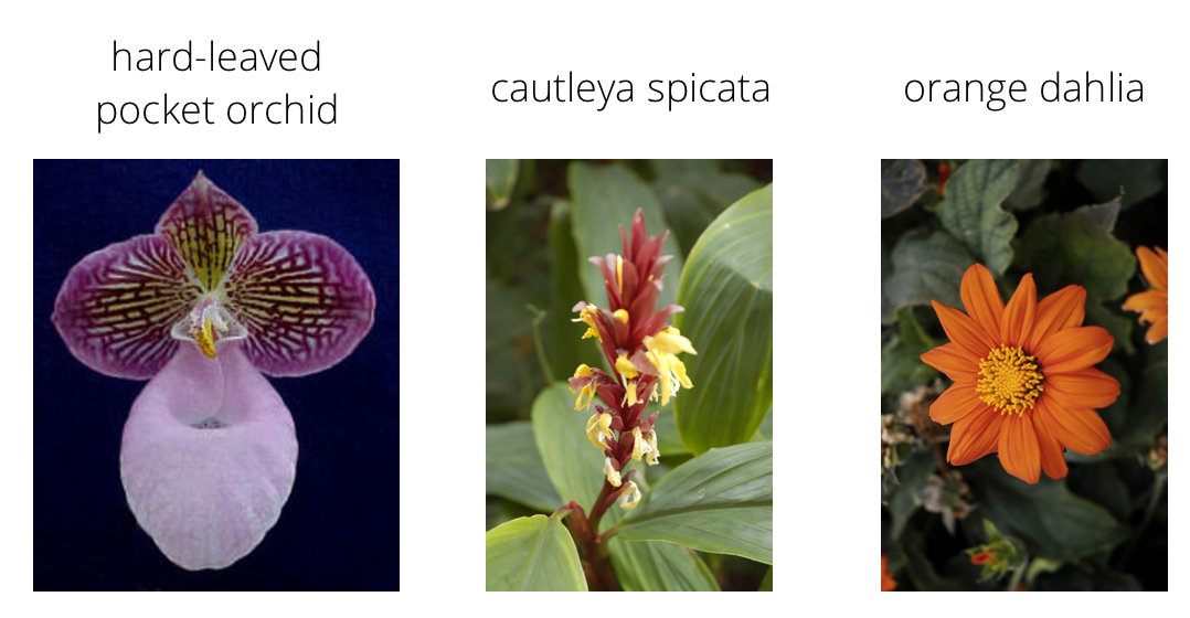
In this project, you’ll train an image classifier to recognize different species of flowers. You can imagine using something like this in a phone app that tells you the name of the flower your camera is looking at. In practice you’d train this classifier, then export it for use in your application. We’ll be using this dataset of 102 flower categories, you can see a few examples below.
The project is broken down into multiple steps:
- Load and preprocess the image dataset
- Train the image classifier on your dataset
- Use the trained classifier to predict image content
We’ll lead you through each part which you’ll implement in Python.
When you’ve completed this project, you’ll have an application that can be trained on any set of labeled images. Here your network will be learning about flowers and end up as a command line application. But, what you do with your new skills depends on your imagination and effort in building a dataset. For example, imagine an app where you take a picture of a car, it tells you what the make and model is, then looks up information about it. Go build your own dataset and make something new.
First up is importing the packages you’ll need. It’s good practice to keep all the imports at the beginning of your code. As you work through this notebook and find you need to import a package, make sure to add the import up here.
# Imports here
%matplotlib inline
%config InlineBackend.figure_format = 'retina'

import matplotlib.pyplot as plt
import seaborn as sns
import numpy as np
from PIL import Image
from collections import OrderedDict

import torch
from torch import nn
from torch import optim
from torchvision import datasets, transforms, models
import torch.nn.functional as F
from torch.optim import lr_scheduler
from torch.autograd import Variable
Load the data
Here you’ll use torchvision to load the data (documentation). The data should be included alongside this notebook, otherwise you can download it here. The dataset is split into three parts, training, validation, and testing. For the training, you’ll want to apply transformations such as random scaling, cropping, and flipping. This will help the network generalize leading to better performance. You’ll also need to make sure the input data is resized to 224x224 pixels as required by the pre-trained networks.
The validation and testing sets are used to measure the model’s performance on data it hasn’t seen yet. For this you don’t want any scaling or rotation transformations, but you’ll need to resize then crop the images to the appropriate size.
The pre-trained networks you’ll use were trained on the ImageNet dataset where each color channel was normalized separately. For all three sets you’ll need to normalize the means and standard deviations of the images to what the network expects. For the means, it’s [0.485, 0.456, 0.406] and for the standard deviations [0.229, 0.224, 0.225], calculated from the ImageNet images. These values will shift each color channel to be centered at 0 and range from -1 to 1.
Setup directories
The Udacity dataset comes with images in the following directory structure:
- root
- dataset ie.. training, validation, and test
- category or class (102 of them. ie… different flower species)
- image file name
/flowers/train/category/image.jpg
Here we setup variables so we can access each dataset.
data_dir = 'flowers'
train_dir = data_dir + '/train'
valid_dir = data_dir + '/valid'
test_dir = data_dir + '/test'
Transforms
We then need to transform the data in order to train against it. Transforming is basically a fancy way to say we are adjusting the images to make them more easily trained against.
These transforms methods are part of the pytorch library, and can be imported by running from torchvision import datasets, transforms, models.
Below, we apply the following transformations:
ToTensor: Converts the image to a pytorch tensorRandomHorizontalFlip: Flips the image to give more variety to the networkRandomReziedCrop: Crops the image to size 224 x 224 pixelsNormalize: Sets the color channel for each pixel to somewhere between -1 and 1.
Load datasets
Next, we use ImageFolder and DataLoader to load our data into training, validation, and testing datasets. As it loads the data, it performs the previously defined transforms on the images.
# TODO: Define your transforms for the training, validation, and testing sets
data_transforms = {
    'training' : transforms.Compose([transforms.RandomResizedCrop(224),
                                    transforms.RandomHorizontalFlip(),transforms.RandomRotation(30),
                                    transforms.ToTensor(),
                                    transforms.Normalize([0.485, 0.456, 0.406],
                                                         [0.229, 0.224, 0.225])]),

    'validation' : transforms.Compose([transforms.Resize(256),
                                      transforms.CenterCrop(224),
                                      transforms.ToTensor(),
                                      transforms.Normalize([0.485, 0.456, 0.406],
                                                           [0.229, 0.224, 0.225])]),

    'testing' : transforms.Compose([transforms.Resize(256),
                                      transforms.CenterCrop(224),
                                      transforms.ToTensor(),
                                      transforms.Normalize([0.485, 0.456, 0.406],
                                                           [0.229, 0.224, 0.225])])
}


# TODO: Load the datasets with ImageFolder
image_datasets = {
    'training' : datasets.ImageFolder(train_dir, transform=data_transforms['training']),
    'testing' : datasets.ImageFolder(test_dir, transform=data_transforms['testing']),
    'validation' : datasets.ImageFolder(valid_dir, transform=data_transforms['validation'])
}

# TODO: Using the image datasets and the trainforms, define the dataloaders
dataloaders = {
    'training' : torch.utils.data.DataLoader(image_datasets['training'], batch_size=64, shuffle=True),
    'testing' : torch.utils.data.DataLoader(image_datasets['testing'], batch_size=64, shuffle=False),
    'validation' : torch.utils.data.DataLoader(image_datasets['validation'], batch_size=64, shuffle=True)
}

class_to_idx = image_datasets['training'].class_to_idx
Label mapping
You’ll also need to load in a mapping from category label to category name. You can find this in the file cat_to_name.json. It’s a JSON object which you can read in with the json module. This will give you a dictionary mapping the integer encoded categories to the actual names of the flowers.
# Provided by Udacity
import json

with open('cat_to_name.json', 'r') as f:
    cat_to_name = json.load(f)
# Quick test
cat_to_name['1']
'pink primrose'
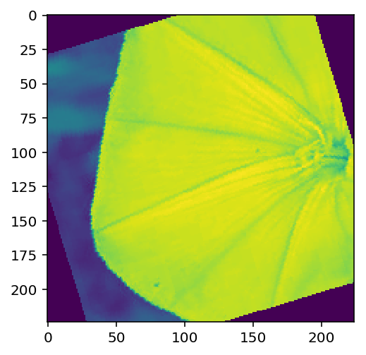
Now we can check that each image can be loaded correctly. We use a generator and iterator to spit out the images one at a time, since we don’t want to load the entire dataset into memory.
images, labels = next(iter(dataloaders["training"]))
print(len(images[0,2]))
plt.imshow(images[0,0])
224


<matplotlib.image.AxesImage at 0x7f6048fc5518>
Building and training the classifier
Now that the data is ready, it’s time to build and train the classifier. As usual, you should use one of the pretrained models from torchvision.models to get the image features. Build and train a new feed-forward classifier using those features.
Transfer learning
Rather than building a model and training from scratch, we can leverage a pretrained model, and adjust the classifier (the last part of it) as needed to fit our needs. This saves a huge amount of time and effort. You can see below, that after we import vgg19 model, we can type model and it will display the architecture. The ‘features’ are what we want to keep, and the ‘classifer’ is what we will change. I initially wanted to use Resnet34, but I didn’t see any option to split up the features and the classifer. So VGG19 it is.
# Transfer learning with VGG19
model = models.vgg19(pretrained=True)
Downloading: "https://download.pytorch.org/models/vgg19-dcbb9e9d.pth" to /root/.torch/models/vgg19-dcbb9e9d.pth
100%|██████████| 574673361/574673361 [00:10<00:00, 55242048.93it/s]
model
VGG(
  (features): Sequential(
    (0): Conv2d(3, 64, kernel_size=(3, 3), stride=(1, 1), padding=(1, 1))
    (1): ReLU(inplace)
    (2): Conv2d(64, 64, kernel_size=(3, 3), stride=(1, 1), padding=(1, 1))
    (3): ReLU(inplace)
    (4): MaxPool2d(kernel_size=2, stride=2, padding=0, dilation=1, ceil_mode=False)
    (5): Conv2d(64, 128, kernel_size=(3, 3), stride=(1, 1), padding=(1, 1))
    (6): ReLU(inplace)
    (7): Conv2d(128, 128, kernel_size=(3, 3), stride=(1, 1), padding=(1, 1))
    (8): ReLU(inplace)
    (9): MaxPool2d(kernel_size=2, stride=2, padding=0, dilation=1, ceil_mode=False)
    (10): Conv2d(128, 256, kernel_size=(3, 3), stride=(1, 1), padding=(1, 1))
    (11): ReLU(inplace)
    (12): Conv2d(256, 256, kernel_size=(3, 3), stride=(1, 1), padding=(1, 1))
    (13): ReLU(inplace)
    (14): Conv2d(256, 256, kernel_size=(3, 3), stride=(1, 1), padding=(1, 1))
    (15): ReLU(inplace)
    (16): Conv2d(256, 256, kernel_size=(3, 3), stride=(1, 1), padding=(1, 1))
    (17): ReLU(inplace)
    (18): MaxPool2d(kernel_size=2, stride=2, padding=0, dilation=1, ceil_mode=False)
    (19): Conv2d(256, 512, kernel_size=(3, 3), stride=(1, 1), padding=(1, 1))
    (20): ReLU(inplace)
    (21): Conv2d(512, 512, kernel_size=(3, 3), stride=(1, 1), padding=(1, 1))
    (22): ReLU(inplace)
    (23): Conv2d(512, 512, kernel_size=(3, 3), stride=(1, 1), padding=(1, 1))
    (24): ReLU(inplace)
    (25): Conv2d(512, 512, kernel_size=(3, 3), stride=(1, 1), padding=(1, 1))
    (26): ReLU(inplace)
    (27): MaxPool2d(kernel_size=2, stride=2, padding=0, dilation=1, ceil_mode=False)
    (28): Conv2d(512, 512, kernel_size=(3, 3), stride=(1, 1), padding=(1, 1))
    (29): ReLU(inplace)
    (30): Conv2d(512, 512, kernel_size=(3, 3), stride=(1, 1), padding=(1, 1))
    (31): ReLU(inplace)
    (32): Conv2d(512, 512, kernel_size=(3, 3), stride=(1, 1), padding=(1, 1))
    (33): ReLU(inplace)
    (34): Conv2d(512, 512, kernel_size=(3, 3), stride=(1, 1), padding=(1, 1))
    (35): ReLU(inplace)
    (36): MaxPool2d(kernel_size=2, stride=2, padding=0, dilation=1, ceil_mode=False)
  )
  (classifier): Sequential(
    (0): Linear(in_features=25088, out_features=4096, bias=True)
    (1): ReLU(inplace)
    (2): Dropout(p=0.5)
    (3): Linear(in_features=4096, out_features=4096, bias=True)
    (4): ReLU(inplace)
    (5): Dropout(p=0.5)
    (6): Linear(in_features=4096, out_features=1000, bias=True)
  )
)
In the classifier, the first line (0): Linear(in_features=25088) indicates that it’s expecting 25088 inputs into the first layer. When we define our own classifier below, we will keep this input size. However, we will need to adjust the last output to match the number of categories we have. In this case 102 flower species. We use ReLU activation functions at each hidden layer, and then apply a Softmax loss function to calculate error.
classifier = nn.Sequential(OrderedDict([
                          ('fc1', nn.Linear(25088, 4096)), # First layer
                          ('relu', nn.ReLU()), # Apply activation function
                          ('fc2', nn.Linear(4096, 102)), # Output layer
                          ('output', nn.LogSoftmax(dim=1)) # Apply loss function
                          ]))
We don’t want to udpate the weights of our pretrained model, just the classifier. So we can use the following code:
for param in model.parameters():
    param.requires_grad = False
Next, we replace the classifier in the model with the one we just built.
model.classifier = classifier
Training
Now we want to train the final layers of the model. The following functions will run forward and backward propogation with pytorch against the training set, and then test against the validation set.
The primary inputs are:
model: this specifies the model we defined earlier. Vgg16, with our custom classifier.epoch: number of full passes through the network (forward and backward).learning_rate: controls how fast the network learns.criterion: used to evaluate error. Associated with loss function that we decide to use.optimizer: which flavor of gradient descent to use
def train(model, epochs, learning_rate, criterion, optimizer, training_loader, validation_loader):

    model.train() # Puts model into training mode
    print_every = 40
    steps = 0
    use_gpu = False

    # Check to see whether GPU is available
    if torch.cuda.is_available():
        use_gpu = True
        model.cuda()
    else:
        model.cpu()

    # Iterates through each training pass based on #epochs & GPU/CPU
    for epoch in range(epochs):
        running_loss = 0
        for inputs, labels in iter(training_loader):
            steps += 1

            if use_gpu:
                inputs = Variable(inputs.float().cuda())
                labels = Variable(labels.long().cuda())
            else:
                inputs = Variable(inputs)
                labels = Variable(labels)

            # Forward and backward passes
            optimizer.zero_grad() # zero's out the gradient, otherwise will keep adding
            output = model.forward(inputs) # Forward propogation
            loss = criterion(output, labels) # Calculates loss
            loss.backward() # Calculates gradient
            optimizer.step() # Updates weights based on gradient & learning rate
            running_loss += loss.item()

            if steps % print_every == 0:
                validation_loss, accuracy = validate(model, criterion, validation_loader)

                print("Epoch: {}/{} ".format(epoch+1, epochs),
                        "Training Loss: {:.3f} ".format(running_loss/print_every),
                        "Validation Loss: {:.3f} ".format(validation_loss),
                        "Validation Accuracy: {:.3f}".format(accuracy))
Notes on backprop:
-
loss.backward()- computes dloss/dx for every parameter x which has requires_grad=True. These are accumulated into x.grad for every parameter x. In pseudo-code:x.grad += dloss/dx -
optimizer.stepupdates the value of x using the gradient x.grad. For example, the SGD optimizer performs:x += -lr * x.grad -
optimizer.zero_grad()clears x.grad for every parameter x in the optimizer. It’s important to call this before loss.backward(), otherwise you’ll accumulate the gradients from multiple passes. -
optimizer.step()updates the weights.
def validate(model, criterion, data_loader):
    model.eval() # Puts model into validation mode
    accuracy = 0
    test_loss = 0

    for inputs, labels in iter(data_loader):
        if torch.cuda.is_available():
            inputs = Variable(inputs.float().cuda(), volatile=True)
            labels = Variable(labels.long().cuda(), volatile=True)
        else:
            inputs = Variable(inputs, volatile=True)
            labels = Variable(labels, volatile=True)

        output = model.forward(inputs)
        test_loss += criterion(output, labels).item()
        ps = torch.exp(output).data
        equality = (labels.data == ps.max(1)[1])
        accuracy += equality.type_as(torch.FloatTensor()).mean()

    return test_loss/len(data_loader), accuracy/len(data_loader)
Testing your network
It’s good practice to test your trained network on test data, images the network has never seen either in training or validation. This will give you a good estimate for the model’s performance on completely new images. Run the test images through the network and measure the accuracy, the same way you did validation. You should be able to reach around 70% accuracy on the test set if the model has been trained well.
Set the following inputs based on what we documented above. Train the network!
epochs = 9
learning_rate = 0.001
criterion = nn.NLLLoss()
optimizer = optim.Adam(model.classifier.parameters(), lr=learning_rate)
train(model, epochs, learning_rate, criterion, optimizer, dataloaders['training'], dataloaders['validation'])
/opt/conda/envs/fastai/lib/python3.6/site-packages/ipykernel_launcher.py:8: UserWarning: volatile was removed and now has no effect. Use `with torch.no_grad():` instead.

/opt/conda/envs/fastai/lib/python3.6/site-packages/ipykernel_launcher.py:9: UserWarning: volatile was removed and now has no effect. Use `with torch.no_grad():` instead.
  if __name__ == '__main__':


Epoch: 1/9  Training Loss: 5.795  Validation Loss: 2.442  Validation Accuracy: 0.395
Epoch: 1/9  Training Loss: 8.011  Validation Loss: 1.424  Validation Accuracy: 0.610
Epoch: 2/9  Training Loss: 0.616  Validation Loss: 1.140  Validation Accuracy: 0.678
Epoch: 2/9  Training Loss: 2.087  Validation Loss: 0.949  Validation Accuracy: 0.731
Epoch: 2/9  Training Loss: 3.336  Validation Loss: 0.850  Validation Accuracy: 0.765
Epoch: 3/9  Training Loss: 1.017  Validation Loss: 0.661  Validation Accuracy: 0.813
Epoch: 3/9  Training Loss: 2.204  Validation Loss: 0.615  Validation Accuracy: 0.819
Epoch: 4/9  Training Loss: 0.280  Validation Loss: 0.696  Validation Accuracy: 0.813
Epoch: 4/9  Training Loss: 1.283  Validation Loss: 0.725  Validation Accuracy: 0.795
Epoch: 4/9  Training Loss: 2.348  Validation Loss: 0.678  Validation Accuracy: 0.821
Epoch: 5/9  Training Loss: 0.681  Validation Loss: 0.622  Validation Accuracy: 0.829
Epoch: 5/9  Training Loss: 1.651  Validation Loss: 0.583  Validation Accuracy: 0.835
Epoch: 6/9  Training Loss: 0.122  Validation Loss: 0.570  Validation Accuracy: 0.854
Epoch: 6/9  Training Loss: 0.990  Validation Loss: 0.588  Validation Accuracy: 0.840
Epoch: 6/9  Training Loss: 1.872  Validation Loss: 0.573  Validation Accuracy: 0.847
Epoch: 7/9  Training Loss: 0.488  Validation Loss: 0.578  Validation Accuracy: 0.838
Epoch: 7/9  Training Loss: 1.311  Validation Loss: 0.611  Validation Accuracy: 0.835
Epoch: 7/9  Training Loss: 2.137  Validation Loss: 0.550  Validation Accuracy: 0.854
Epoch: 8/9  Training Loss: 0.849  Validation Loss: 0.592  Validation Accuracy: 0.841
Epoch: 8/9  Training Loss: 1.693  Validation Loss: 0.513  Validation Accuracy: 0.849
Epoch: 9/9  Training Loss: 0.328  Validation Loss: 0.575  Validation Accuracy: 0.849
Epoch: 9/9  Training Loss: 1.082  Validation Loss: 0.567  Validation Accuracy: 0.842
Epoch: 9/9  Training Loss: 1.879  Validation Loss: 0.653  Validation Accuracy: 0.843
This took about 15-20 mins to train. Also, kind of strange that the training loss is higher than the validation loss. Typically, you would expect training loss to be lower than validation loss, since the model has seen the training images more times.
Save the checkpoint
Now that your network is trained, save the model so you can load it later for making predictions. You probably want to save other things such as the mapping of classes to indices which you get from one of the image datasets: image_datasets['train'].class_to_idx. You can attach this to the model as an attribute which makes inference easier later on.
model.class_to_idx = image_datasets['train'].class_to_idx
Remember that you’ll want to completely rebuild the model later so you can use it for inference. Make sure to include any information you need in the checkpoint. If you want to load the model and keep training, you’ll want to save the number of epochs as well as the optimizer state, optimizer.state_dict. You’ll likely want to use this trained model in the next part of the project, so best to save it now.
model.class_to_idx = image_datasets['training'].class_to_idx
model.cpu()
torch.save({'arch': 'vgg19',
            'state_dict': model.state_dict(), # Holds all the weights and biases
            'class_to_idx': model.class_to_idx},
            'classifier.pth')
Loading the checkpoint
At this point it’s good to write a function that can load a checkpoint and rebuild the model. That way you can come back to this project and keep working on it without having to retrain the network.
Loading a pretrained network also allows us to run on CPU rather than GPU.
def load_model(checkpoint_path):
    checkpoint = torch.load(checkpoint_path)

    model = models.vgg19(pretrained=True)

    for param in model.parameters():
        param.requires_grad = False

    model.class_to_idx = checkpoint['class_to_idx']

    classifier = nn.Sequential(OrderedDict([
                          ('fc1', nn.Linear(25088, 4096)),
                          ('relu', nn.ReLU()),
                          ('fc2', nn.Linear(4096, 102)),
                          ('output', nn.LogSoftmax(dim=1))
                          ]))

    model.classifier = classifier

    model.load_state_dict(checkpoint['state_dict'])

    return model
model = load_model('classifier.pth')
model
VGG(
  (features): Sequential(
    (0): Conv2d(3, 64, kernel_size=(3, 3), stride=(1, 1), padding=(1, 1))
    (1): ReLU(inplace)
    (2): Conv2d(64, 64, kernel_size=(3, 3), stride=(1, 1), padding=(1, 1))
    (3): ReLU(inplace)
    (4): MaxPool2d(kernel_size=2, stride=2, padding=0, dilation=1, ceil_mode=False)
    (5): Conv2d(64, 128, kernel_size=(3, 3), stride=(1, 1), padding=(1, 1))
    (6): ReLU(inplace)
    (7): Conv2d(128, 128, kernel_size=(3, 3), stride=(1, 1), padding=(1, 1))
    (8): ReLU(inplace)
    (9): MaxPool2d(kernel_size=2, stride=2, padding=0, dilation=1, ceil_mode=False)
    (10): Conv2d(128, 256, kernel_size=(3, 3), stride=(1, 1), padding=(1, 1))
    (11): ReLU(inplace)
    (12): Conv2d(256, 256, kernel_size=(3, 3), stride=(1, 1), padding=(1, 1))
    (13): ReLU(inplace)
    (14): Conv2d(256, 256, kernel_size=(3, 3), stride=(1, 1), padding=(1, 1))
    (15): ReLU(inplace)
    (16): Conv2d(256, 256, kernel_size=(3, 3), stride=(1, 1), padding=(1, 1))
    (17): ReLU(inplace)
    (18): MaxPool2d(kernel_size=2, stride=2, padding=0, dilation=1, ceil_mode=False)
    (19): Conv2d(256, 512, kernel_size=(3, 3), stride=(1, 1), padding=(1, 1))
    (20): ReLU(inplace)
    (21): Conv2d(512, 512, kernel_size=(3, 3), stride=(1, 1), padding=(1, 1))
    (22): ReLU(inplace)
    (23): Conv2d(512, 512, kernel_size=(3, 3), stride=(1, 1), padding=(1, 1))
    (24): ReLU(inplace)
    (25): Conv2d(512, 512, kernel_size=(3, 3), stride=(1, 1), padding=(1, 1))
    (26): ReLU(inplace)
    (27): MaxPool2d(kernel_size=2, stride=2, padding=0, dilation=1, ceil_mode=False)
    (28): Conv2d(512, 512, kernel_size=(3, 3), stride=(1, 1), padding=(1, 1))
    (29): ReLU(inplace)
    (30): Conv2d(512, 512, kernel_size=(3, 3), stride=(1, 1), padding=(1, 1))
    (31): ReLU(inplace)
    (32): Conv2d(512, 512, kernel_size=(3, 3), stride=(1, 1), padding=(1, 1))
    (33): ReLU(inplace)
    (34): Conv2d(512, 512, kernel_size=(3, 3), stride=(1, 1), padding=(1, 1))
    (35): ReLU(inplace)
    (36): MaxPool2d(kernel_size=2, stride=2, padding=0, dilation=1, ceil_mode=False)
  )
  (classifier): Sequential(
    (fc1): Linear(in_features=25088, out_features=4096, bias=True)
    (relu): ReLU()
    (fc2): Linear(in_features=4096, out_features=102, bias=True)
    (output): LogSoftmax()
  )
)
Notice our updated classifier now shows up in the (classifier) section identified above.
Inference for classification
Now you’ll write a function to use a trained network for inference. That is, you’ll pass an image into the network and predict the class of the flower in the image. Write a function called predict that takes an image and a model, then returns the top $K$ most likely classes along with the probabilities. It should look like
probs, classes = predict(image_path, model)
print(probs)
print(classes)
> [ 0.01558163  0.01541934  0.01452626  0.01443549  0.01407339]
> ['70', '3', '45', '62', '55']
First you’ll need to handle processing the input image such that it can be used in your network.
Image Preprocessing
You’ll want to use PIL to load the image (documentation). It’s best to write a function that preprocesses the image so it can be used as input for the model. This function should process the images in the same manner used for training.
First, resize the images where the shortest side is 256 pixels, keeping the aspect ratio. This can be done with the thumbnail or resize methods. Then you’ll need to crop out the center 224x224 portion of the image.
Color channels of images are typically encoded as integers 0-255, but the model expected floats 0-1. You’ll need to convert the values. It’s easiest with a Numpy array, which you can get from a PIL image like so np_image = np.array(pil_image).
As before, the network expects the images to be normalized in a specific way. For the means, it’s [0.485, 0.456, 0.406] and for the standard deviations [0.229, 0.224, 0.225]. You’ll want to subtract the means from each color channel, then divide by the standard deviation.
And finally, PyTorch expects the color channel to be the first dimension but it’s the third dimension in the PIL image and Numpy array. You can reorder dimensions using ndarray.transpose. The color channel needs to be first and retain the order of the other two dimensions.
I picked a random folder and image, set it to the image_path below. Then displayed the image for reference.
image_path = test_dir + '/34/image_06961.jpg'
img = Image.open(image_path)
img
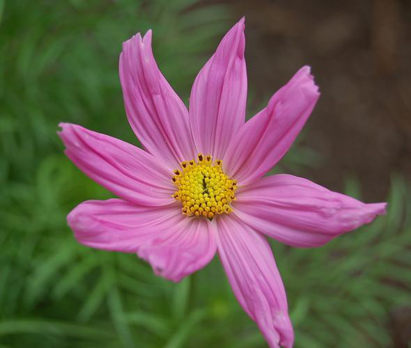
Check the current image size.
img.size
(590, 500)
I’m using the same transforms code from above to define a function for processing individual images. By using the transforms method, it will turn the image into a tensor. We will need to change it back to an array later on.
def process_image(image_path):
    img = Image.open(image_path)
    adjust = transforms.Compose([transforms.Resize(256),
                                      transforms.CenterCrop(224),
                                      transforms.ToTensor(),
                                      transforms.Normalize([0.485, 0.456, 0.406],
                                                           [0.229, 0.224, 0.225])])
    img_tensor = adjust(img)

    return img_tensor
Process the image identified above with the process_image() function I just created.
processed_image = process_image(image_path)
Check to see that the image was transformed into the appropriate tensor shape. 3 color channels, 224 pixels by 224 pixels. I accidentally imported a .PNG file rather than .JPG file, and it gave me 4 color channels. My tensor shape was 4, 224, 224, and I got a ValueError: operands could not be broadcast together with shapes (224, 224, 4) (3,). Make sure to use a jpg file.
processed_image.shape
torch.Size([3, 224, 224])
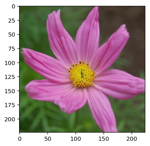
To check your work, the function below converts a PyTorch tensor and displays it in the notebook. If your process_image function works, running the output through this function should return the original image (except for the cropped out portions).
This function is provided by Udacity.
def imshow(image, ax=None, title=None):
    """Imshow for Tensor."""
    if ax is None:
        fig, ax = plt.subplots()

    # PyTorch tensors assume the color channel is the first dimension
    # but matplotlib assumes is the third dimension
    image = image.numpy().transpose((1, 2, 0))

    # Undo preprocessing
    mean = np.array([0.485, 0.456, 0.406])
    std = np.array([0.229, 0.224, 0.225])
    image = std * image + mean

    # Image needs to be clipped between 0 and 1 or it looks like noise when displayed
    image = np.clip(image, 0, 1)

    ax.imshow(image)

    return ax
Shows that the image was processed correctly.
imshow(processed_image)
<matplotlib.axes._subplots.AxesSubplot at 0x7f6020b5b0b8>
Class Prediction
Once you can get images in the correct format, it’s time to write a function for making predictions with your model. A common practice is to predict the top 5 or so (usually called top-$K$) most probable classes. You’ll want to calculate the class probabilities then find the $K$ largest values.
To get the top $K$ largest values in a tensor use x.topk(k). This method returns both the highest k probabilities and the indices of those probabilities corresponding to the classes. You need to convert from these indices to the actual class labels using class_to_idx which hopefully you added to the model or from an ImageFolder you used to load the data (see here). Make sure to invert the dictionary so you get a mapping from index to class as well.
Again, this method should take a path to an image and a model checkpoint, then return the probabilities and classes.
probs, classes = predict(image_path, model)
print(probs)
print(classes)
> [ 0.01558163  0.01541934  0.01452626  0.01443549  0.01407339]
> ['70', '3', '45', '62', '55']
Now we need to show the top 5 predictions. The first argument we need to pass to our model is batch size. So we need to use processed_image.unsqeeze(0) to set the first argument to 1 (since there is only 1 image). The new shape of our tensor is (1, 3, 224, 224).
processed_image = process_image(image_path)
processed_image.unsqueeze_(0)
tensor([[[[-1.1932, -1.2103, -1.2617,  ..., -1.0390, -1.0562, -1.0904],
          [-1.1932, -1.1932, -1.2445,  ..., -1.0390, -1.0562, -1.0733],
          [-1.1932, -1.1760, -1.1760,  ..., -1.0390, -1.0562, -1.0904],
          ...,
          [-1.2788, -1.2788, -1.2959,  ..., -0.9020, -0.8678, -0.8849],
          [-1.1589, -1.1589, -1.2103,  ..., -0.9020, -0.8678, -0.8507],
          [-1.0562, -1.0904, -1.1247,  ..., -0.9020, -0.8849, -0.8507]],

         [[-0.6527, -0.6527, -0.6352,  ..., -1.1429, -1.1604, -1.1954],
          [-0.6877, -0.6702, -0.6527,  ..., -1.1429, -1.1604, -1.1954],
          [-0.7227, -0.7052, -0.6702,  ..., -1.1429, -1.1604, -1.2129],
          ...,
          [-0.6176, -0.6001, -0.6001,  ..., -0.7227, -0.6877, -0.6176],
          [-0.4951, -0.4951, -0.4601,  ..., -0.6702, -0.6527, -0.6527],
          [-0.3901, -0.4076, -0.3901,  ..., -0.6527, -0.6527, -0.6527]],

         [[-1.2816, -1.2641, -1.2641,  ..., -1.1073, -1.1247, -1.1247],
          [-1.2293, -1.2119, -1.2467,  ..., -1.1247, -1.1421, -1.1421],
          [-1.1944, -1.1770, -1.2467,  ..., -1.1247, -1.1421, -1.1421],
          ...,
          [-1.2816, -1.2816, -1.2990,  ..., -1.0376, -1.0027, -0.9853],
          [-1.0898, -1.1073, -1.1596,  ..., -1.0376, -1.0201, -0.9853],
          [-0.9853, -1.0201, -1.0550,  ..., -1.0201, -1.0201, -0.9853]]]])
Next we get the top probabilities from the output of our model, then assign them along with labels to top_probs and top_labs.
probs = torch.exp(model.forward(processed_image))
top_probs, top_labs = probs.topk(5)
top_probs
tensor([[9.9998e-01, 1.3435e-05, 4.7965e-06, 4.4158e-08, 3.8500e-08]],
       grad_fn=<TopkBackward>)
top_labs
tensor([[30, 57, 46, 68, 47]])
Now we switch the key and values of the index_to_class dictionary so we can pull the indexes based on the class.
idx_to_class = {}
for key, value in model.class_to_idx.items():
    idx_to_class[value] = key
Convert to numpy array.
np_top_labs = top_labs[0].numpy()
np_top_labs[0]
30
top_labels = []
for label in np_top_labs:
    top_labels.append(int(idx_to_class[label]))
top_labels
[34, 59, 49, 69, 5]
Now we have our top labels. But it makes more sense to show flower names.
top_flowers2 = [cat_to_name[str(lab)] for lab in top_labels]
top_flowers2
['mexican aster',
 'orange dahlia',
 'oxeye daisy',
 'windflower',
 'english marigold']
We put everything together in the function below:
def predict(image_path, model, topk=5):
    ''' Predict the class (or classes) of an image using a trained deep learning model.
    '''

    processed_image = process_image(image_path)
    processed_image.unsqueeze_(0)
    probs = torch.exp(model.forward(processed_image))
    top_probs, top_labs = probs.topk(topk)

    idx_to_class = {}
    for key, value in model.class_to_idx.items():
        idx_to_class[value] = key

    np_top_labs = top_labs[0].numpy()

    top_labels = []
    for label in np_top_labs:
        top_labels.append(int(idx_to_class[label]))

    top_flowers = [cat_to_name[str(lab)] for lab in top_labels]

    return top_probs, top_labels, top_flowers
Run our prediction!
predict(image_path, model, topk=5)
(tensor([[9.9998e-01, 1.3435e-05, 4.7965e-06, 4.4158e-08, 3.8500e-08]],
        grad_fn=<TopkBackward>),
 [34, 59, 49, 69, 5],
 ['mexican aster',
  'orange dahlia',
  'oxeye daisy',
  'windflower',
  'english marigold'])
Sanity Checking
Now that you can use a trained model for predictions, check to make sure it makes sense. Even if the testing accuracy is high, it’s always good to check that there aren’t obvious bugs. Use matplotlib to plot the probabilities for the top 5 classes as a bar graph, along with the input image. It should look like this:
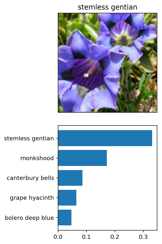
You can convert from the class integer encoding to actual flower names with the cat_to_name.json file (should have been loaded earlier in the notebook). To show a PyTorch tensor as an image, use the imshow function defined above.
def plot_solution(image_path, model):
    # Sets up our plot
    plt.figure(figsize = (6,10))
    ax = plt.subplot(2,1,1)
    # Set up title
    flower_num = image_path.split('/')[2]
    title_ = cat_to_name[flower_num] # Calls dictionary for name
    # Plot flower
    img = process_image(image_path)
    plt.title(title_)
    imshow(img, ax)
    # Make prediction
    top_probs, top_labels, top_flowers = predict(image_path, model)
    top_probs = top_probs[0].detach().numpy() #converts from tensor to nparray
    # Plot bar chart
    plt.subplot(2,1,2)
    sns.barplot(x=top_probs, y=top_flowers, color=sns.color_palette()[0]);
    plt.show()

    print(top_probs, top_labels, top_flowers)
plot_solution(image_path, model)
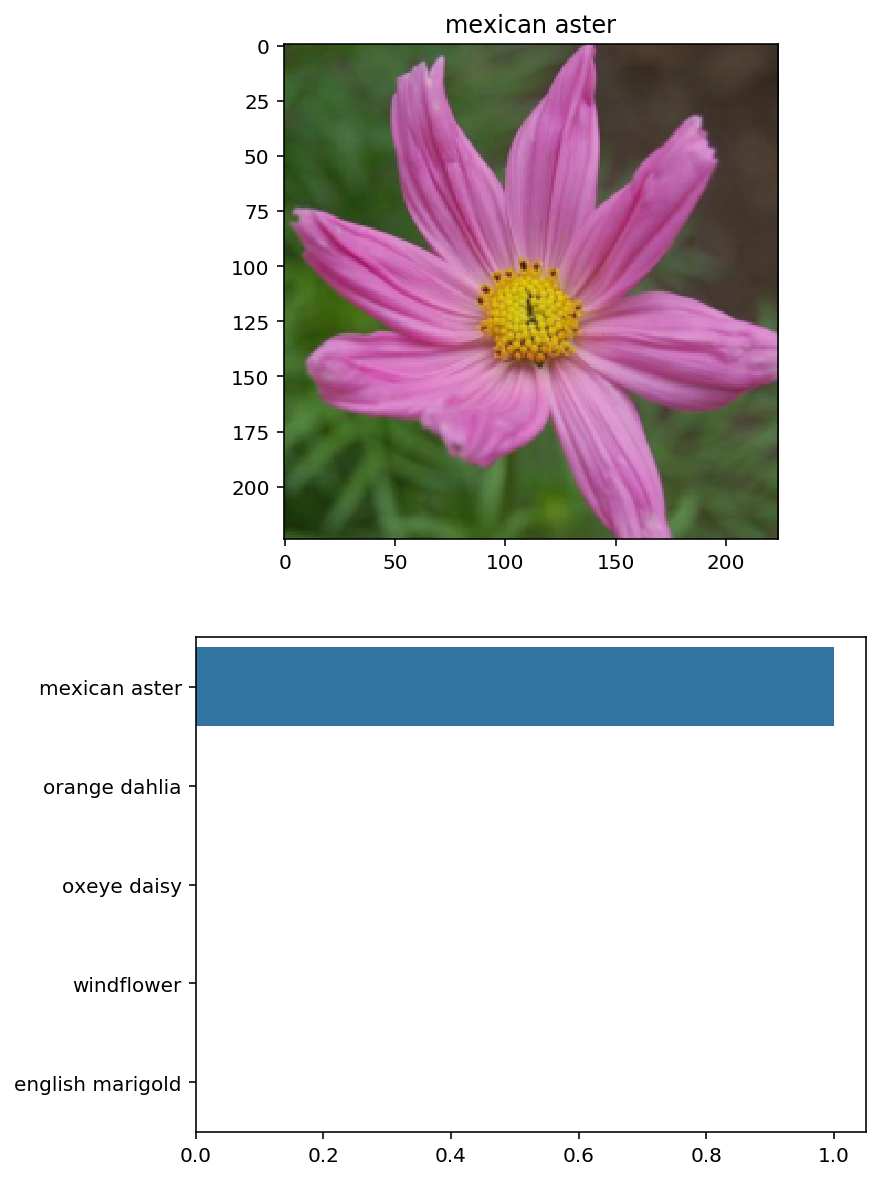
[9.9998093e-01 1.3435291e-05 4.7964527e-06 4.4157503e-08 3.8499653e-08] [34, 59, 49, 69, 5] ['mexican aster', 'orange dahlia', 'oxeye daisy', 'windflower', 'english marigold']
Let’s try with a different flower:
# Try with 45/image_07139.jpg
image_path = test_dir + '/45/image_07139.jpg'
plot_solution(image_path, model)
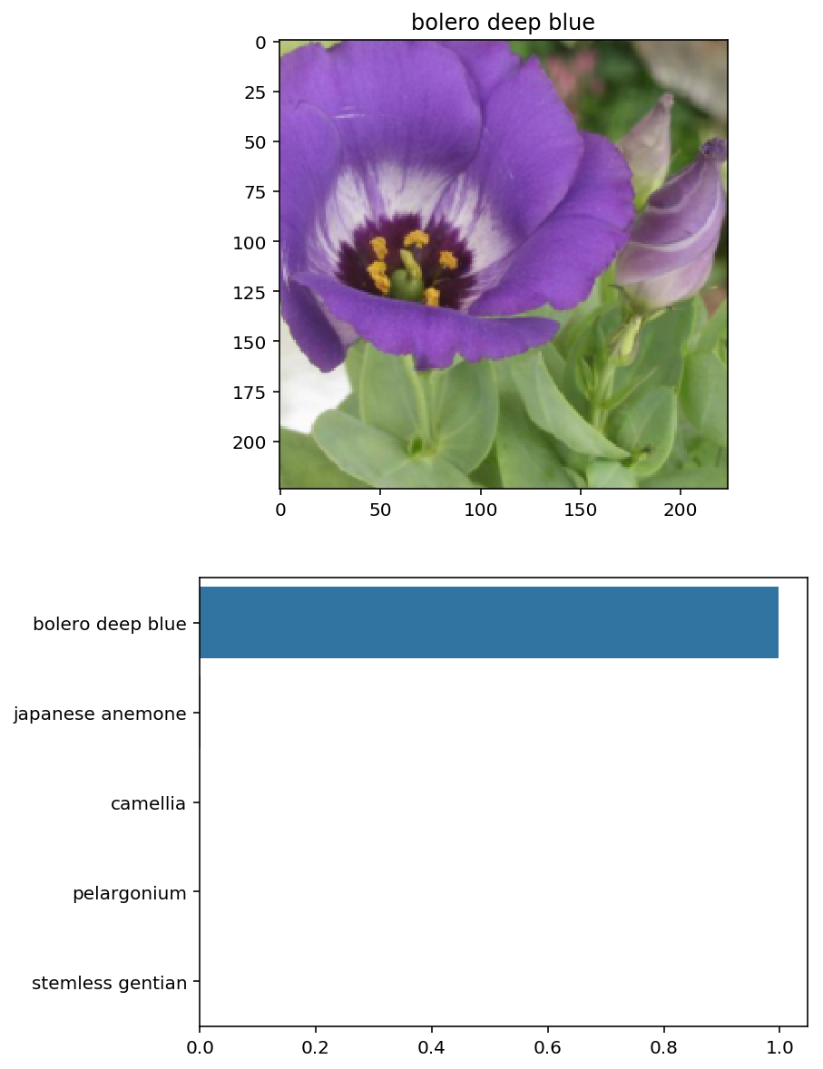
[9.9756348e-01 1.2083625e-03 4.1649581e-04 2.0346409e-04 1.3860803e-04] [45, 62, 96, 55, 28] ['bolero deep blue', 'japanese anemone', 'camellia', 'pelargonium', 'stemless gentian']
This project took me about 20 hours to complete, and 60 hours overall for the entire nanodegree. I referred to a lot of the Udacity materials provided in the Pytorch lessons. I also had to do a lot of Googling to get an idea for how to start. I also wanted to credit Josh Bernhard for inspiring me to turn this into a blog post. His post was a great resource, and provided a lot of guidance when I got stuck.