Quantitative Value
I recently read the book Quantitative Value, written by Wes Gray, and Tobias Carlisle. It’s a strategy that takes a systematic approach to value investing.
In a previous post, I talked about Warren Buffet and his quote “It’s far better to buy a wonderful company at a fair price than a fair company at a wonderful price."
This isn’t as easy as it sounds, so I was curious to find out if there were any ways for us regular investors to identify wonderful companies at fair prices. Quantitative Value explores this concept in more detail.
One of the examples touched upon in the book is Joel Greenblatt’s Magic Formula. The Magic Formula uses ROIC to determine if a company is ‘wonderful’, and uses Earnings Yield (EBIT / Enterprise Value), to determine whether the price is fair. The Magic Formula strategy tells you to rank companies based on the combination of these two ratios, and systematically buy the top ranked ones, with periodic rebalances. Backtests have shown this approach to consistently beat the market.
Alternatively, in the book The Acquirer’s Multiple (also authored by Tobias Carlisle), Carlisle shows that eliminating ROIC and only looking at EV-to-Operating Income (which is EBIT stated from a top down approach) actually provides higher returns than the Magic Formula.
His thesis states that buying fair companies at wonderful prices is better than buying wonderful companies at fair prices.
This is also demonstrated in Quantitative Value, where Gray and Carlisle show how EV-to-EBIT, along with a handful of other quantitative metrics can be used to deliver market beating returns.
I wanted to reproduce the backtest results, so I implemented a simplified version using some of the key factors in Quantitative Value. I wasn’t able to apply every item on the checklist, but I did get positive results by doing the following:
- Start with universe of tradeable stocks in the US with Market cap > 500M
- Screen out all companies in financial, real estate and utilities sectors
- Screen out potential manipulators
- Screen out financially distressed companies
- Identify wonderful prices by ranking companies by EV-to-EBIT
- Buy 30 ‘cheapest’ companies based on EV-to-EBIT each month
- Rebalance on a monthly basis, sell once the companies are not longer in screen
- Run backtest from 1/3/2007 - 9/28/2018
Summary of Results
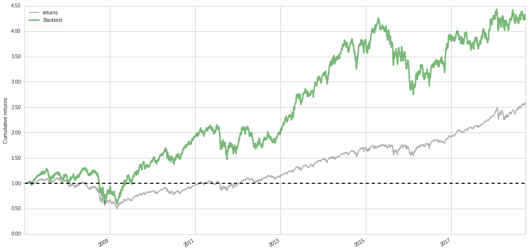
Cumulative returns for the period were 323.8% (green line), compared to 157.8% for the S&P500 benchmark (gray line), and annual returns of 13% and 8.4% respectively. From a risk adjusted standpoint, the Quantitative Value portfolio had a slightly higher Sharpe ratio compared to the benchmark, which is a positive sign. However, the beta for the portfolio is 1.18, indicating a higher volatility relative to the market. I’m not sure how representative of a test this is, but it was fun to try and replicate the results from the book. Below is a more detailed summary of how the algorithm performed against the S&P500, Russell1000, and Russell3000 from 2007 - 2018.
| QV Algo | SPY Benchmark | Russell 1000 | Russell 3000 | |
|---|---|---|---|---|
| Cumulative Returns | 323.81% | 157.87% | 150.98% | 149.12% |
| Annual Returns | 13.09% | 8.41% | 8.16% | 8.09% |
| Annual Volatility | 26.19% | 19.38% | 19.34% | 19.73% |
| Sharpe Ratio | 0.60 | 0.51 | 0.50 | 0.49 |
| Sortino Ratio | 0.85 | 0.72 | 0.70 | 0.69 |
| Max Drawdown | -54.72% | -54.88% | -56.20% | -56.44% |
| Alpha | 0.04 | 0.00 | 0.00 | 0.00 |
| Beta | 1.18 | 1.00 | 0.99 | 1.01 |
| Start Date | 2007-01-03 | |||
| End date | 2018-09-28 | |||
| Total Months | 140 |
Here’s a comparison of annual returns between the algorithm and the Acquirer’s Multiple strategy (200M and up market cap). I would expect very similar results, since they are both heavily reliant on screening with EV-to-EBIT.
| Annual Returns | QV Algo | Acquirer’s Multiple | S&P500 |
|---|---|---|---|
| 2007 | 16.4% | -10.0% | 5.5% |
| 2008 | -20.1% | -32.1% | -37.0% |
| 2009 | 61.0% | 66.2% | 26.5% |
| 2010 | 32.5% | 39.4% | 15.1% |
| 2011 | -8.0% | -11.5% | 2.1% |
| 2012 | 18.6% | 14.3% | 16.0% |
| 2013 | 47.2% | 42.1% | 32.4% |
| 2014 | 1.18% | 1.4% | 13.7% |
| 2015 | -11.2% | -6.6% | 1.4% |
| 2016 | 15.9% | 21.9% | 12.0% |
| 2017 | 11.8% | -2.8% (Q1 Only) | 19.9% |
| 2018 | 1.5% | n/a | 10.6% |
My Algorithm
I chose Quantopian as the platform to build my algorithm. Primarily because I took the Python for Financial Analysis and Algorithmic Trading course on Udemy, and Quantopian was the platform they used. I found Quantopian useful because they have a robust backtesting library along with free access to data. This meant I could focus on the algorithm itself, rather than trying to setup my own environment.
Quantopian provides quite a few free educational resources on algo trading. To learn more about how to use their platform go here.
For those interested, below is a breakdown of my algorithm.
Initialize & schedule
This first part imports the libraries needed for the algorithm. The initialize function is called when the algorithm first runs. The schedule_function() is called here to determine how often to trade. In this case, The algorithm runs once at at the end of each month, one hour after the market opens. The attach_pipeline() function attaches our pipeline of stocks to this algorithm. The pipeline is basically the screen I have created to determine which stocks to trade.
# Import libraries
import quantopian.algorithm as algo
from quantopian.pipeline.filters import QTradableStocksUS
from quantopian.pipeline.domain import US_EQUITIES
from quantopian.pipeline import Pipeline
from quantopian.pipeline.data.factset import Fundamentals
from quantopian.pipeline.factors.fundamentals import MarketCap
import quantopian.pipeline.data.morningstar as mstar

# Initialize
def initialize(context):
    """
    Called once at the start of the algorithm.
    """
    # Rebalance every month, 1 hour after market open.
    algo.schedule_function(
        rebalance,
        algo.date_rules.month_end(),
        algo.time_rules.market_open(hours=1),
    )

    # Create our dynamic stock selector.
    algo.attach_pipeline(make_pipeline(), 'pipeline')
Define factors and filter universe of stocks
The make_pipeline() function is where all the logic is for determining which stocks make it into the screen. This is where I have reproduced the rules defined in Quantitative Value. make_pipeline() walks through the following set of criteria:
Start with universe of tradeable stocks in the US with Market cap > 500M
- Uses Quantopian’s built in QTradeableStocksUS filter
Screen out all companies in financial, real estate and utilities sectors
- These sectors have very different business models relative to most companies
- Uses Morningstar
Fundamentals.morningstar_sector_codeto screen out sectors
Screen out potential manipulators
-
Gray and Carlisle highlight how accounting accruals are a common source of financial statement manipulation. In the book, they use Scaled Total Accruals (STA), and Scaled Net Operating Assets (SNOA) as a way to identify potential manipulators. These are calculated as:
STA = (Net Income - CF from operations) / Total AssetsSNOA = (Operating Assets - Operating Liabilities) / Total Assets -
Next, rank the entire universe of companies based on the STA and SNOA scores, and take the average to calculate a Combined Accrual Ranking.
-
Finally, filter out the companies which ranked in the highest 95th percentile of the Combined Accrual Ranking.
Screen out financially distressed companies
- Use the Altman Z-score bankruptcy predictor to screen out all stocks with a score below 1.81.
Identify wonderful prices by ranking companies by EV-to-EBIT
- This is essentially the Acquirer’s Multiple.
- Filter out all companies with EV-to-EBIT above 10. The lower number the better.
- Filter out all companies with a negative EV-to-EBIT
def make_pipeline():
    """
    A function to create our dynamic stock selector (pipeline). Documentation
    on pipeline can be found here:
    https://www.quantopian.com/help#pipeline-title
    """

    base_universe = QTradableStocksUS

    # Get fundamental data
    ev_to_ebit = Fundamentals.entrpr_val_ebit_oper_qf.latest
    net_income = Fundamentals.net_inc_af.latest
    cf_from_op = Fundamentals.oper_cf_af.latest
    total_assets = Fundamentals.assets.latest
    cash = Fundamentals.cash_generic_af.latest
    st_debt = Fundamentals.debt_st_tot_af.latest
    lt_debt = Fundamentals.debt_lt_tot_af.latest
    min_interest = Fundamentals.min_int_accum.latest
    preferred_stock = Fundamentals.pfd_stk.latest
    common_equity = Fundamentals.com_eq.latest
    z_score = Fundamentals.zscore_af.latest

    # Calc Scaled Total Accruals
    sta = (net_income - cf_from_op) / total_assets

    # Calc Scaled net operating assets
    op_assets = total_assets - cash
    op_liabilities = (total_assets - st_debt - lt_debt -
                      min_interest - preferred_stock - common_equity)
    snoa = (op_assets - op_liabilities) / total_assets

    # Calc P_STA & P_SNOA
    p_sta = sta.rank()
    p_snoa = snoa.rank()

    # Calc combo_accrual ranks
    accrual_rank = (p_sta + p_snoa) / 2

    # Filter out high percentile of combo accruals > 95th
    # Keep the 0-95 percentile
    accrual_filter = accrual_rank.percentile_between(0,95)

    # Filter for acquirers multiple
    pos_ent_ebit = ev_to_ebit > 0
    high_ent_ebit = ev_to_ebit < 10

    # Filter out low z_score
    z_score_filter = z_score > 1.81

    # Filter out real estate, financials, utilities sectors
    excluded_sectors = [103,104,207]
    sector = mstar.Fundamentals.morningstar_sector_code.latest


    # Set filters
    tradeable_stocks = (pos_ent_ebit
                    & high_ent_ebit
                    & accrual_filter
                    & z_score_filter
                    & base_universe())

    sector_filter = ~sector.element_of(excluded_sectors)

    pipe = Pipeline(columns={'EV to Ebit':ev_to_ebit},
                  domain=US_EQUITIES,screen=(tradeable_stocks & sector_filter))
    return pipe
Execute trades
Buy 30 ‘cheapest’ companies based on EV-to-EBIT each month
-
Once the pipeline of stocks has been created, the
before_trading_start()function will take the pipeline output, and create a list of the top 30 stocks on our screener to purchase. -
The
rebalance()function executes on a monthly basis, and opens equal weighted long positions of the top 30 stocks in the list.
Rebalance on a monthly basis, sell once the companies are no longer in screen
- The
rebalance()function also closes positions on any stocks in our portfolio that are no longer showing up on our trading list.
def before_trading_start(context, data):
    """
    Called every day before market open.
    """
    context.output = algo.pipeline_output('pipeline')

    # These are the securities that we are interested in trading each day.
    # Creates list of securities with 30 smallest EV to Ebit number
    context.security_list = context.output.nsmallest(30, 'EV to Ebit').index.tolist()


def rebalance(context, data):
    """
    Execute orders according to our schedule_function() timing.
    """
    trading_list = context.security_list
    new_positions = 0
    target_percentage = .033

    # Close positions if no longer in AM screener
    for security in context.portfolio.positions:
        if security not in trading_list:
            order_target_percent(security,0)

    # Open positions for securities in AM screener
    for security in trading_list:
        order_target_percent(security,target_percentage)
Conclusion
Overall, I’m fairly happy with the results. One interesting finding was the high portfolio beta, even though the Sharpe ratio was higher than the market. Makes me wonder if the strategy is just banking on high volatility associated with ‘cheap’ stocks to generate retruns. Modern portfolio theory equates volatility to risk, but as a value investor, I’m not entirely sold on that concept.
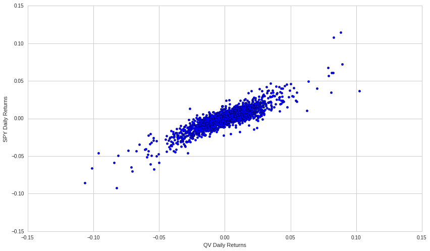
My algorithm also highly correlated with the market. I calculated its correlation coefficient to be 0.869! If you look at the chart below comparing Quantitative Value portfolio returns vs. SPY Market returns, you can see a direct linear relationship. This further contributes to my assessment that perhaps this strategy is just taking advantage of volatility to generate above market returns.
For reference, here are the backtest results directly from the Quantitative Value book, comparing the QV strategy to the market, as well as other funds. I wasn’t able to reproduce all the factors in my algorithm, so this likely explains the divergence in results.
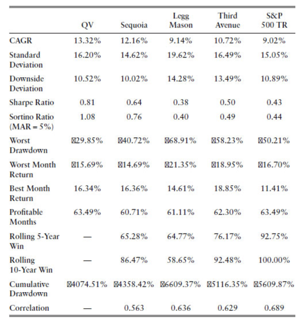 Source: Quantitative Value - Gray & Carlisle
That just about wraps it up. This was a great learning exercise, and I’m looking forward to experimenting with some more quantitative investing strategies.