These are my notes from the book Grokking Deep Learning by Andrew Trask. Feel free to check my first post on this book to get my overall thoughts and recommendations on how to approach this series. The rest of my notes for this book can be found here

Time to simplify

Impractical to think about everything all the time

Use mental tools. This chapter focuses on the construction of efficient concepts in your mind.

What have we learned so far?

• Idea of machine learning in general
• How individual linear nodes (neurons) learn
• Horizontal groups of neurons (layers)
• Vertical groups (stacks of layers)
• Learning is just reducing error to 0
• Use calculus to discover how to change each weight in network to move error in direction of 0.

All of the previous lessons lead to a single idea:

• Neural networks search for (and create) correlation between input and output datasets.

To prevent us from being overwhelemed by the complexity of deep learning, let’s hold on to this idea of correlation, rather than all the previous smaller ideas. Call it correlation summarization

Correlation summarization

Correlation summarization - At the 10,000 foot level:

“Neural networks seek to find direct and indirect correlation between an input layer and an output layer, which are determined by the input and output datasets, respectively."

Local correlation summarization - What if only 2 layers?

“Any given set of weights optimizes to learn how to correlate its input layer with what the output layer says it should be."

Global correlation summarization - Backpropogation

“What an earlier layer says it should be can be determined by taking what a later layer says it should be and multiplying it by the weights in between them. This way, later layers can tell earlier layers what kind of signal they need, to ultimately find correlation with the output. This cross-communication is called backpropogation."

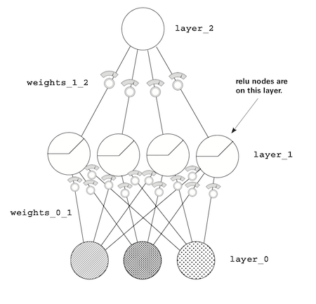
Previously overcomplicated visualization

Rather than looking at each layer in detail, Adam wants us to now focus on the concept of correlation summarization. In the previous visualization:

• Weights are matrices (weights_0_1, weights_1_2)
• Layers are vectors (layer_0, layer_1, layer_2)

The simplified visualization

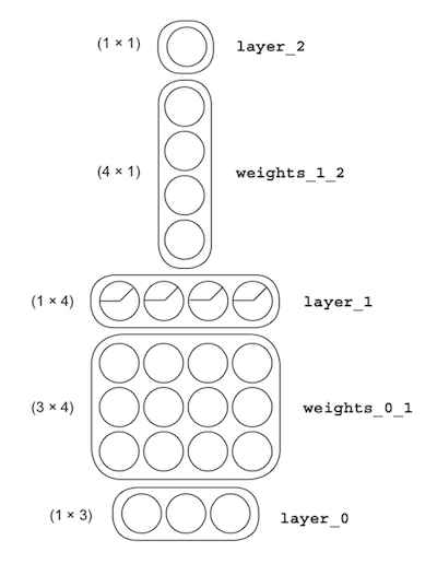
Think of neural networks as LEGO bricks, with each brick representing a vector or matrix. In the image below, the strips are vectors, and blocks are matrices.

Simplifying even further

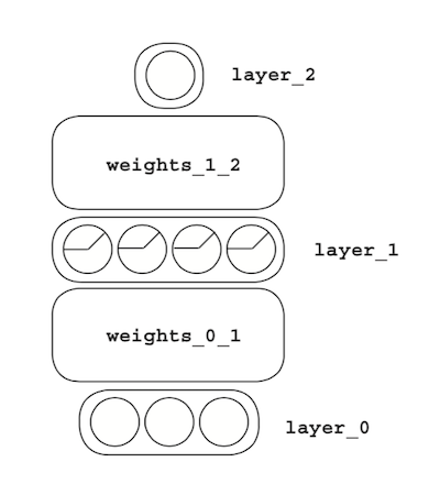
The number of dimensions in a matrix is determined by the layers. Each matrix’s number of rows and columns has a direct relationship to the dimensions of the layers before and after them.

Going back to this example, we can infer that weights_0_1 is a 3x4 matrix because layer_0 has three dimensions, and layer_1 has four dimensions.

This neural network will adjust the weights to find correlation between layer_0 and layer_2. The different configurations of weights and layers will have a strong impact on determining success at finding correlation.

The specific confguratino of weights and layers in a network is called its architecture.

Visualizing using letters instead of pictures

We can use simple algebra to explain what’s happening in these pictures. Let’s label each component of the network like this:

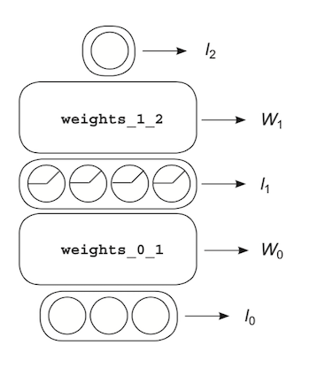
Let’s label layers with lowercase l, and weights with uppercase W. Then put a little subscript next to it so we know which layer or weight it’s referring to.

Linking the variables

Now we can combine the letters to indicate functions and operations.

Vector-matrix multiplication

• Take layer 0 vector, and perform vector matrix multiplication with weight matrix 0: $$l _ { 0 }W _ { 0 }$$

• Same thing, but using layer vector 1 and weight matrix 1: $$l _ { 1 }W _ { 1 }$$

Create assignments, and apply functions:

• Create layer 1 by taking layer 0 vector, and perform vector matrix multiplication with weight matrix 0. Then perform relu function on the output: $$l _ { 1 } = relu(l _ { 0 }W _ { 0 })$$

• Create layer 2 by taking layer 1 vector and perform vector matrix multiplication against weight matrix 1: $$l _ { 2 } = l _ { 1 } W _ { 1 }$$

All together in 1 line!

$$l _ { 2 } = r e l u \left( l _ { 0 } W _ { 0 } \right) W _ { 1 }$$

Everything side by side

Here’s the visualization, algebra formula, and Python code all together for forward propogation!

Python

layer_2 = relu(layer_0.dot(weights_0_1)).dot(weights_1_2)

Algebra

$$l _ { 2 } = r e l u \left( l _ { 0 } W _ { 0 } \right) W _ { 1 }$$

Visualization

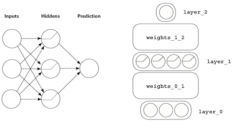
Key takeaway

“Good neural architectures channel signal so that correlation is easy to discover. Great architectures also filter noise to prevent overfitting."