.::howieko::.
Stuff that I'm learning
For this project, we will build another image classifer using the same flowers dataset from our last project. Our model will perform fine grain classification to identify 102 species of flowers. Instead of using just Pytorch, this classifier is built using the Fastai library.
Import libraries
%reload_ext autoreload
%autoreload 2
%matplotlib inline

# Import fastai library

from fastai.vision import *
from fastai.metrics import error_rate
from pathlib import Path
Note: It’s not best praxtice to use import * when importing libraries. In this example however, we are aiming for a more interactive/experimental approach. So not necessarily following PEP8 standards. Different style of coding. Rules are a little different with datascience. Most important thing is to interactively experiment quickly.
Load data
The folder structure is the same as from our last project, with a training set, validation set, and test set. Each class / category has a folder name between 1-102
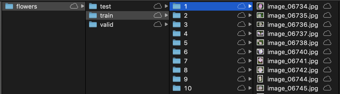
path = Path('flowers')
path.ls()
[PosixPath('flowers/valid'),
 PosixPath('flowers/export.pkl'),
 PosixPath('flowers/train'),
 PosixPath('flowers/models'),
 PosixPath('flowers/flower_data.tar'),
 PosixPath('flowers/test')]
path_valid = path/'valid'
path_train = path/'train'
path_test = path/'test'
bs = 64 # Set batch size
Everything you model with is going to be a Fastai databunch object. This object contains our training set, validation set, and testing set.
Similar to what we did with torchvision transforms, we need to adjust our images so they can be trained on.
Set image sizes: GPU has to apply exact same instruction for things at the same time in order to be fast. If images are different shapes / sizes, it can’t do it. We need to make all the images the same size.
Use size = 224 x 224. Generally works for most things.
Normalize the data - make it the same size.. ie, same mean & standard dev. Pixel values range from 0-255. Some channels might be really bright, or not bright. Normalizing will set each of the channels to be a mean of 0, and standard deviation of 1. Makes it easier for the model to train well.
data = ImageDataBunch.from_folder(path, ds_tfms=get_transforms(), size=224, bs=bs
                                  ).normalize(imagenet_stats)
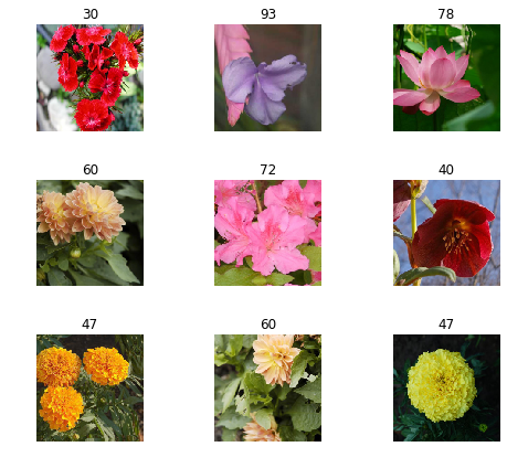
Let’s take a look at the images:
data.show_batch(rows=3, figsize=(7,6))
Take a look at all the labels. In the case of our dataset, they are based on the folder names for each flowers species.
print(data.classes)

print(len(data.classes), data.c) # .c is number of classes for classification problems
['1', '10', '100', '101', '102', '11', '12', '13', '14', '15', '16', '17', '18', '19', '2', '20', '21', '22', '23', '24', '25', '26', '27', '28', '29', '3', '30', '31', '32', '33', '34', '35', '36', '37', '38', '39', '4', '40', '41', '42', '43', '44', '45', '46', '47', '48', '49', '5', '50', '51', '52', '53', '54', '55', '56', '57', '58', '59', '6', '60', '61', '62', '63', '64', '65', '66', '67', '68', '69', '7', '70', '71', '72', '73', '74', '75', '76', '77', '78', '79', '8', '80', '81', '82', '83', '84', '85', '86', '87', '88', '89', '9', '90', '91', '92', '93', '94', '95', '96', '97', '98', '99']
102 102
Numbers as folder names don’t really give us meaningful information. In this case, I think it would be better if we converted these numbers to the actual flower names. This will also be much more useful once we try validating some of our predictions later on.
Luckily, Udacity provides a dictionary mapping of folder names to flower names.
# Provided by Udacity
import json

with open('cat_to_name.json', 'r') as f:
    cat_to_name = json.load(f)
# Lookup first entry:
cat_to_name['1']
'pink primrose'
And here we use os.rename() to perform the actual renaming of the folders.
import os

for key, value in cat_to_name.items():
    os.rename(path_valid/key, path_valid/value)
# checking our work
!ls flowers/valid
alpine sea holly      fire lily               peruvian lily
anthurium             foxglove                petunia
artichoke             frangipani              pincushion flower
azalea                fritillary              pink primrose
ball moss             garden phlox            pink-yellow dahlia
balloon flower        gaura                   poinsettia
barbeton daisy        gazania                 primula
bearded iris          geranium                prince of wales feathers
bee balm              giant white arum lily   purple coneflower
bird of paradise      globe thistle           red ginger
bishop of llandaff    globe-flower            rose
black-eyed susan      grape hyacinth          ruby-lipped cattleya
blackberry lily       great masterwort        siam tulip
blanket flower        hard-leaved pocket orchid  silverbush
bolero deep blue      hibiscus                snapdragon
bougainvillea         hippeastrum             spear thistle
bromelia              japanese anemone        spring crocus
buttercup             king protea             stemless gentian
californian poppy     lenten rose             sunflower
camellia              lotus lotus             sweet pea
canna lily            love in the mist        sweet william
canterbury bells      magnolia                sword lily
cape flower           mallow                  thorn apple
carnation             marigold                tiger lily
cautleya spicata      mexican aster           toad lily
clematis              mexican petunia         tree mallow
colt's foot           monkshood               tree poppy
columbine             moon orchid             trumpet creeper
common dandelion      morning glory           wallflower
corn poppy            orange dahlia           water lily
cyclamen              osteospermum            watercress
daffodil              oxeye daisy             wild pansy
desert-rose           passion flower          windflower
english marigold      pelargonium             yellow iris
Cool! It worked! Now, let’s do the same thing for our training and test sets.
for key, value in cat_to_name.items():
    os.rename(path_train/key, path_train/value)
    os.rename(path_test/key, path_test/value)
Look at our classes again. This time with the updated names:
print(data.classes)

print(len(data.classes), data.c)
['alpine sea holly', 'anthurium', 'artichoke', 'azalea', 'ball moss', 'balloon flower', 'barbeton daisy', 'bearded iris', 'bee balm', 'bird of paradise', 'bishop of llandaff', 'black-eyed susan', 'blackberry lily', 'blanket flower', 'bolero deep blue', 'bougainvillea', 'bromelia', 'buttercup', 'californian poppy', 'camellia', 'canna lily', 'canterbury bells', 'cape flower', 'carnation', 'cautleya spicata', 'clematis', "colt's foot", 'columbine', 'common dandelion', 'corn poppy', 'cyclamen', 'daffodil', 'desert-rose', 'english marigold', 'fire lily', 'foxglove', 'frangipani', 'fritillary', 'garden phlox', 'gaura', 'gazania', 'geranium', 'giant white arum lily', 'globe thistle', 'globe-flower', 'grape hyacinth', 'great masterwort', 'hard-leaved pocket orchid', 'hibiscus', 'hippeastrum', 'japanese anemone', 'king protea', 'lenten rose', 'lotus lotus', 'love in the mist', 'magnolia', 'mallow', 'marigold', 'mexican aster', 'mexican petunia', 'monkshood', 'moon orchid', 'morning glory', 'orange dahlia', 'osteospermum', 'oxeye daisy', 'passion flower', 'pelargonium', 'peruvian lily', 'petunia', 'pincushion flower', 'pink primrose', 'pink-yellow dahlia', 'poinsettia', 'primula', 'prince of wales feathers', 'purple coneflower', 'red ginger', 'rose', 'ruby-lipped cattleya', 'siam tulip', 'silverbush', 'snapdragon', 'spear thistle', 'spring crocus', 'stemless gentian', 'sunflower', 'sweet pea', 'sweet william', 'sword lily', 'thorn apple', 'tiger lily', 'toad lily', 'tree mallow', 'tree poppy', 'trumpet creeper', 'wallflower', 'water lily', 'watercress', 'wild pansy', 'windflower', 'yellow iris']

102 102
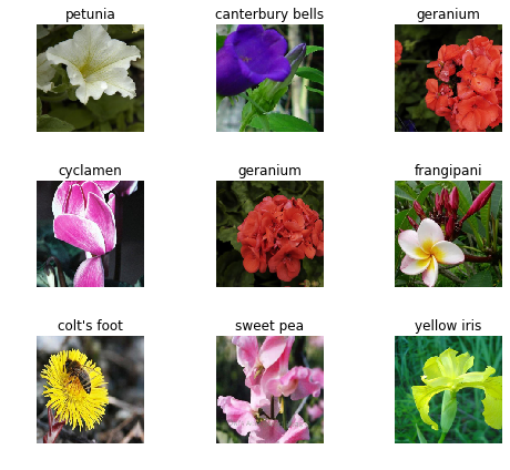
And now we can re-create our ImageDataBunch with the updated labels.
data = ImageDataBunch.from_folder(path, ds_tfms=get_transforms(), size=224, bs=bs
                                  ).normalize(imagenet_stats)
data.show_batch(rows=3, figsize=(7,6))
Training the model
Using transfer learning, we can take a mdoel that knows how to do something pretty well, and make it do what we want it to do really well. We use a pre-trained model, then fit it so that instead of 1000 categories of image net data, it predicts the categories that we want. In this case the 102 species of flowers. Transfer learning allows us to train models with 1/100th less of the time, with thousands of times less of data.
Learner is a Fastai concept that we used to fit models. create_cnn is what we will use to create a convolutional neural network.
data - assigns to a databunch
model - assigns architecture that we are using, in this case ResNet34
Unlike the Udacity project, in which we used the VGG19 architecture, we will use ResNet34 to train our model. In the lecture, somebody asked why we were using ResNet. Jeremey said it was good enough, and referenced the Stanford Dawn Deep Learning benchmarks… top 5 were all ResNet!

So let’s create our model:
learn = create_cnn(data, models.resnet34, metrics=error_rate)
Important to use validation set to check images that the model has not seen before in order to to prevent overfitting. Overfitting is when the model sees the same image so many times, it ends up just memorizing it. Unable to generalize against other images. Fastai is hardcoded to check against a validation set. Follows best practices.
‘One cycle learning’ based on 2018 research paper. Turns out it is a dramatically better approach.
learn.fit_one_cycle(4) # 4 Epochs
Total time: 03:26
| epoch | train_loss | valid_loss | error_rate |
|---|---|---|---|
| 1 | 2.771014 | 0.870605 | 0.178484 |
| 2 | 0.895252 | 0.306605 | 0.069682 |
| 3 | 0.400189 | 0.213900 | 0.050122 |
| 4 | 0.253869 | 0.205599 | 0.041565 |
You can see that it took 3 minutes to train, and after 4 passes (epochs), the model was able to reduce the error rate down to 0.051, which is an accuracy rate of 95.8%.
Compare this to the VGG19 classifier I built in Pytorch for the previous project. Which took 20 minutes to train, and had an accuracy rate of 84.3%.
Saving the checkpoint
This way we don’t have to retrain the network again. We can just reload it later on.
learn.save('flowers_stage-1')
Checking results
Now that we have trained our model, we can pass in the learn object and into our ClassificationInterpretation object to review our results.
interp = ClassificationInterpretation.from_learner(learn)

losses,idxs = interp.top_losses()

#Quick check
len(data.valid_ds)==len(losses)==len(idxs)
True
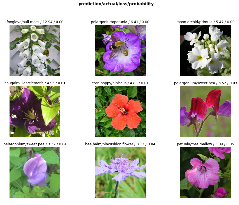
To better understand our predictions, it’s important to identify the things we were the most confident of, that we got wrong. Aka our ‘top losses’.
Use the plot_top_losses function to show images in top_losses along with their prediction, actual, loss, and probability of predicted class.
interp.plot_top_losses(9, figsize=(15,11))
Another useful tool is a ‘confusion matrix’, to get a visual on actuals vs. predicted. Since our model was so accurate however, it just shows a diagonal line across, since the predicted == actuals 96% of the time.
interp.plot_confusion_matrix(figsize=(16,16), dpi=200)
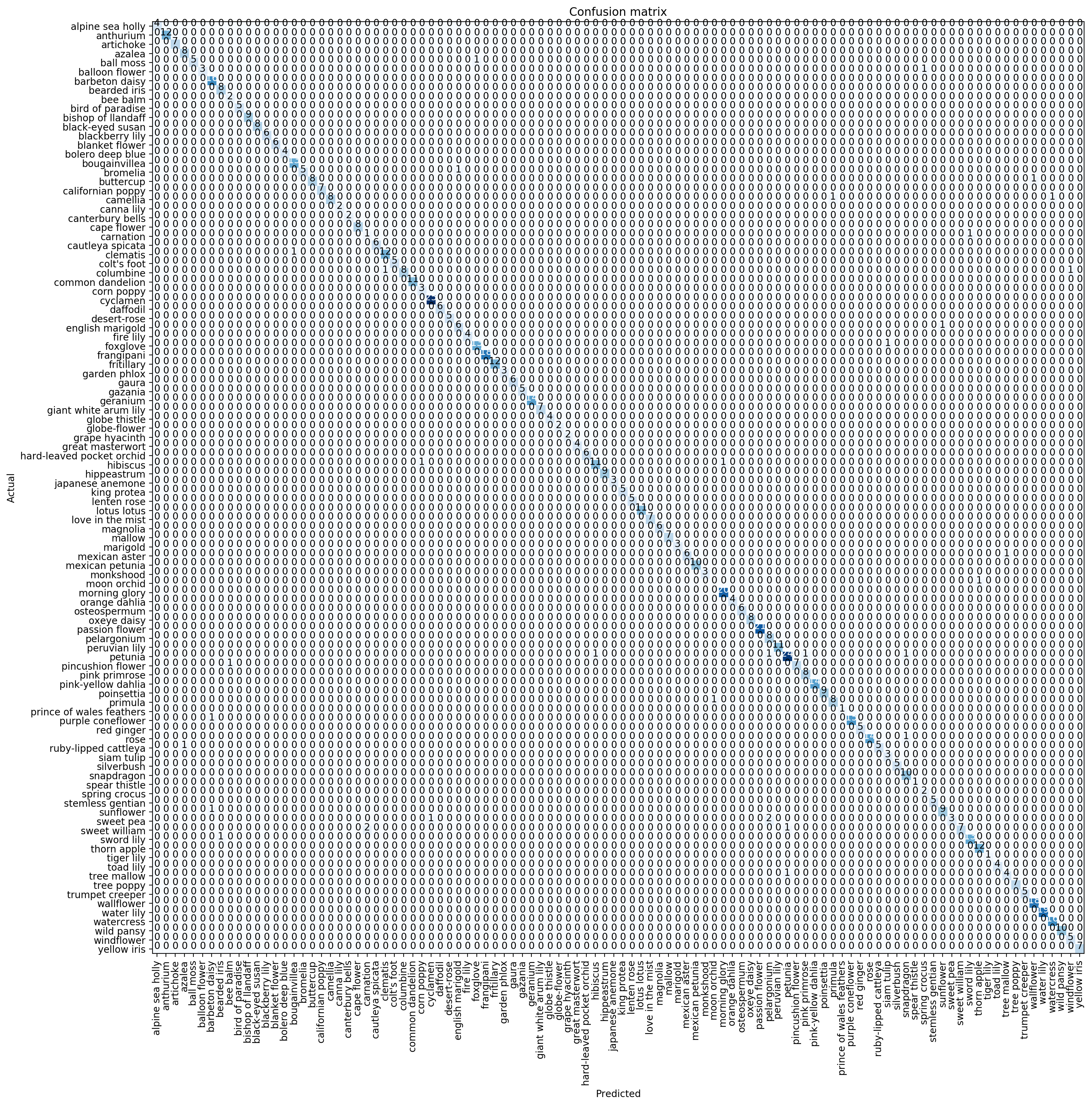
If there are too many classes, it can be hard to read. In that case, use most_confused to print out a summary. Here you can see that ‘sweet william’ was mistaken for ‘carnation’ 2 times, and ‘sweet pea’ was mistaken for ‘pelargonium’ 2 times.
interp.most_confused(min_val=1)
[('sweet pea', 'pelargonium', 2), ('sweet william', 'carnation', 2)]
Here we can see the rest
interp.most_confused(min_val=0)
[('sweet pea', 'pelargonium', 2),
 ('sweet william', 'carnation', 2),
 ('ball moss', 'foxglove', 1),
 ('balloon flower', 'spring crocus', 1),
 ('bromelia', 'english marigold', 1),
 ('buttercup', 'wallflower', 1),
 ('camellia', 'primula', 1),
 ('camellia', 'watercress', 1),
 ('carnation', 'sword lily', 1),
 ('clematis', 'bougainvillea', 1),
 ('columbine', 'clematis', 1),
 ('columbine', 'windflower', 1),
 ('english marigold', 'sunflower', 1),
 ('foxglove', 'siam tulip', 1),
 ('hibiscus', 'corn poppy', 1),
 ('hibiscus', 'morning glory', 1),
 ('mexican aster', 'tree mallow', 1),
 ('moon orchid', 'thorn apple', 1),
 ('petunia', 'hibiscus', 1),
 ('petunia', 'pelargonium', 1),
 ('petunia', 'pink primrose', 1),
 ('petunia', 'snapdragon', 1),
 ('pincushion flower', 'bee balm', 1),
 ('primula', 'moon orchid', 1),
 ('purple coneflower', 'barbeton daisy', 1),
 ('rose', 'snapdragon', 1),
 ('ruby-lipped cattleya', 'azalea', 1),
 ('sunflower', 'barbeton daisy', 1),
 ('sweet pea', 'cyclamen', 1),
 ('sweet william', 'petunia', 1),
 ('sword lily', 'bearded iris', 1),
 ('tree mallow', 'petunia', 1)]
Tweaking our model to make it better
By default, when we run fit_one_cycle Fastai freezes the weights on the model, and only trains on the final few layers of the network (our classifier).
This is similar to what we did in Pytorch with:
for param in model.parameters(): param.requires_grad = False
Since we only wanted our model to train on the classifier.
However, now we are trying to tweak and improve our model, so we can try training on the entire network. This can be done by unfreezing then network using learn.unfreeze()
learn.unfreeze()
learn.fit_one_cycle(2)
Total time: 02:15
| epoch | train_loss | valid_loss | error_rate |
|---|---|---|---|
| 1 | 0.511195 | 0.425937 | 0.117359 |
| 2 | 0.220565 | 0.119531 | 0.028117 |
As we train a convolutional neural network, it’s unlikely that we can get higher accuracy in the first few layers. Since they will likely be just simple shapes, and lines. However, we should do better in the later layers, as they start resemble our images.
Our example actually resulted in a higher level of accuracy!
Loading the checkpoint
Let’s load our previously saved weights, and try some more tweaking.
learn.load('flowers_stage-1')
Learner(data=ImageDataBunch;

Train: LabelList
y: CategoryList (6552 items)
[Category gaura, Category gaura, Category gaura, Category gaura, Category gaura]...
Path: flowers
x: ImageItemList (6552 items)
[Image (3, 500, 752), Image (3, 500, 752), Image (3, 500, 752), Image (3, 500, 667), Image (3, 500, 752)]...
Path: flowers;

Valid: LabelList
y: CategoryList (818 items)
[Category gaura, Category gaura, Category gaura, Category gaura, Category gaura]...
Path: flowers
x: ImageItemList (818 items)
[Image (3, 501, 727), Image (3, 752, 500), Image (3, 500, 752), Image (3, 752, 500), Image (3, 752, 500)]...
Path: flowers;

Test: None, model=Sequential(
  (0): Sequential(
    (0): Conv2d(3, 64, kernel_size=(7, 7), stride=(2, 2), padding=(3, 3), bias=False)
    (1): BatchNorm2d(64, eps=1e-05, momentum=0.1, affine=True, track_running_stats=True)
    (2): ReLU(inplace)
    (3): MaxPool2d(kernel_size=3, stride=2, padding=1, dilation=1, ceil_mode=False)
    (4): Sequential(
      (0): BasicBlock(
        (conv1): Conv2d(64, 64, kernel_size=(3, 3), stride=(1, 1), padding=(1, 1), bias=False)
        (bn1): BatchNorm2d(64, eps=1e-05, momentum=0.1, affine=True, track_running_stats=True)
        (relu): ReLU(inplace)
        (conv2): Conv2d(64, 64, kernel_size=(3, 3), stride=(1, 1), padding=(1, 1), bias=False)
        (bn2): BatchNorm2d(64, eps=1e-05, momentum=0.1, affine=True, track_running_stats=True)
      )
      (1): BasicBlock(
        (conv1): Conv2d(64, 64, kernel_size=(3, 3), stride=(1, 1), padding=(1, 1), bias=False)
        (bn1): BatchNorm2d(64, eps=1e-05, momentum=0.1, affine=True, track_running_stats=True)
        (relu): ReLU(inplace)
        (conv2): Conv2d(64, 64, kernel_size=(3, 3), stride=(1, 1), padding=(1, 1), bias=False)
        (bn2): BatchNorm2d(64, eps=1e-05, momentum=0.1, affine=True, track_running_stats=True)
      )
      .
      .
      .
), Sequential(
  (0): AdaptiveAvgPool2d(output_size=1)
  (1): AdaptiveMaxPool2d(output_size=1)
  (2): Flatten()
  (3): BatchNorm1d(1024, eps=1e-05, momentum=0.1, affine=True, track_running_stats=True)
  (4): Dropout(p=0.25)
  (5): Linear(in_features=1024, out_features=512, bias=True)
  (6): ReLU(inplace)
  (7): BatchNorm1d(512, eps=1e-05, momentum=0.1, affine=True, track_running_stats=True)
  (8): Dropout(p=0.5)
  (9): Linear(in_features=512, out_features=102, bias=True)
)])
Learning rate finder is another Fastai tool. It figures out what is the fastest I can train the network at, without it going off the rails.
learn.lr_find()
LR Finder is complete, type {learner_name}.recorder.plot() to see the graph.
We can plot the learning rate and it’s associated loss.
learn.recorder.plot()
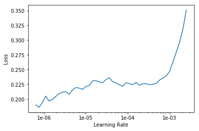
Now let’s re-train the network, this time using the learning rate with the lowest amount of loss.
learn.unfreeze()
learn.fit_one_cycle(4, max_lr=1e-6)
Total time: 04:29
| epoch | train_loss | valid_loss | error_rate |
|---|---|---|---|
| 1 | 0.217776 | 0.204758 | 0.044010 |
| 2 | 0.221629 | 0.200069 | 0.034230 |
| 3 | 0.218738 | 0.197053 | 0.040342 |
| 4 | 0.211052 | 0.197964 | 0.037897 |
It looks like our original training pass was pretty accurate. Even with additional tweaking, I wasn’t able to get the error rate much lower. Compared to the 84% accuracy I got using Pytorch, these are all pretty sweet results.
It’s also possible to set a range for the learning rate. So that it uses a higher rate (learns faster) for the early layers, and then a lower rate (more detailed) for the later layers - where we want to fine tune our model.
By default, fit_one_cycle uses 3e-3 as the learning rate. The range of learning rates would be (start, end), where start is the low point identified by the learning rate finder, and end is the default x 10, or 3e-4. Below is an example:
learn.unfreeze()
learn.fit_one_cycle(4, slice(1e-06, 3e-4))
Total time: 04:30
| epoch | train_loss | valid_loss | error_rate |
|---|---|---|---|
| 1 | 0.220646 | 0.181810 | 0.042787 |
| 2 | 0.174134 | 0.150867 | 0.034230 |
| 3 | 0.136475 | 0.138779 | 0.031785 |
| 4 | 0.114328 | 0.134181 | 0.031785 |
Making Predictions
Inference - When you have a pre-trained model and you are predicting things, this is called inference. Typically when we put our model into production, we are using inference. ie… an App that can take images of flowers, and then look up against pre-trained model to predict species.
Let’s try to predict flower species.
First thing we do is export the content of our Learner object for production:
learn.export()
This will create a file named ‘export.pkl’ in the directory where we were working that contains everything we need to deploy our model (the model, the weights but also some metadata like the classes or the transforms/normalization used).
Typically, we would not need GPU’s for inference. Just CPU’s. To test our model on a CPU, we could run:
defaults.device = torch.device('cpu')
Next, we open an image in Fastai, and assign it to img variable. This could be any image we want to check our predictions against. As long as it is one of the species that we have in our classes.
# Testing with a rose
img = open_image(path_test/'rose/image_01191.jpg')
img

Then we load our learner file. Basically just checking that the export.pkl file we exported earlier is in the right directory.
learn = load_learner(path)
Now let’s make our prediction!
pred_class,pred_idx,outputs = learn.predict(img)
pred_class
Category rose
Success! It accurately predicted a rose!
Let’s try another one…
# Testing with ball moss
img2 = open_image(path_test/'ball moss/image_06021.jpg')
img2
pred_class,pred_idx,outputs = learn.predict(img2)
pred_class
Category ball moss
Right again!
Our model looks pretty accurate! We fed the model some images of a rose, and ball moss from the test directory (which the model has never seen before), and it was able to accurately classify them. Using transfer learning and the Fastai library, we were able to get a 96% accuracy rate, with just 3 minutes of training time! Pretty impressive!